
Introduction
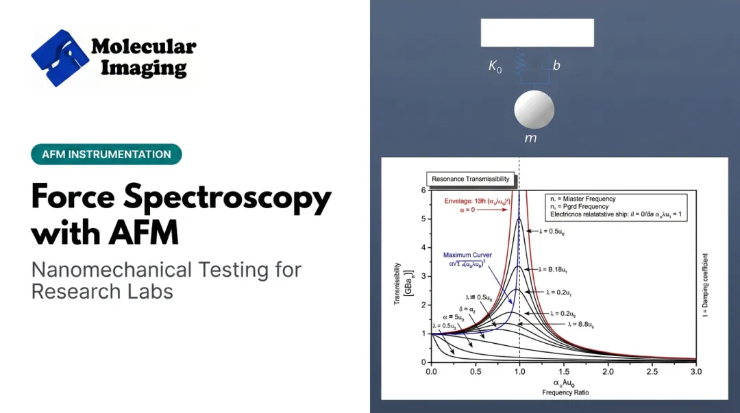
An AFM topography image shows a surface's shape. A force-distance curve tells you what a picture never can: how that surface pushes back. Force spectroscopy lets researchers "feel" a sample at the nanoscale, measuring stiffness, adhesion, and even the moment a single protein unfolds under load.
But force curves are unforgiving. A poorly calibrated cantilever or a rushed contact-point estimate can quietly corrupt every Young's modulus or adhesion value pulled from the data. Many labs discover this only after a reviewer questions their numbers.
The scale of the problem is real. A 2025 study analyzing pooled AFM indentation datasets found researchers rejected nearly 30% of collected curves as anomalous, hours of instrument time spent on data that never made it into a result.
This guide breaks down what force curves actually measure, how to run the workflow correctly, and how to catch artifacts before they enter a dataset.
TL;DR
- Force-distance curves plot tip-sample force vs. probe-sample separation over one approach-retract cycle.
- FD curves quantify Young's modulus, adhesion force, work of adhesion, and single-molecule unfolding events.
- Reliable numbers need calibrated deflection sensitivity, a verified spring constant, and careful contact-point processing.
- Tilted baselines, multiple pull-offs, and transient spikes are common and must be diagnosed, not just discarded blindly.
- Modular BioAFM systems plus hands-on application support shorten setup time and improve force-spectroscopy reliability.
What Is a Force-Distance Curve?
A force-distance (F-D) curve plots cantilever deflection, converted into force, against the vertical position of the probe as it moves toward and away from a sample.
Unlike standard imaging, which scans laterally across a surface, force spectroscopy holds the tip at one XY position and records only the vertical interaction between tip and sample.
That distinction matters. Imaging tells you where features sit on a surface. A force curve tells you what happens the instant the tip touches the material. No topography scan can provide that on its own.
Anatomy of a Force Curve
- Approach: The probe moves toward the surface at a fixed point. The baseline should stay flat; any bending signals long-range attractive or repulsive forces before contact.
- Snap-in (jump-to-contact): Once the attractive force gradient, often capillary or van der Waals in origin, exceeds the cantilever's spring constant, the tip snaps onto the surface.
- Loading (repulsive) segment: The tip pushes into the sample and the cantilever bends upward. This portion feeds directly into stiffness and modulus calculations.
- Retract and pull-off: As the cantilever withdraws, it stays briefly stuck to the surface. The depth and shape of this dip quantify adhesion force and work of adhesion.

Why This Analysis Matters
Force curves yield quantitative data topography alone cannot provide:
- Mechanical properties: Extracted Young's modulus and indentation depth describe stiffness at resolutions no bulk material test can match.
- Adhesion and binding forces: Researchers have measured individual antibody-antigen unbinding events at 244 ± 22 pN, a force far too small for any bulk assay to detect.
- Single-molecule unfolding: Sequential unfolding of protein domains, such as titin, reveals mechanical behavior directly tied to biological function.
- Artifact prevention: Cross-checking force data against topography helps separate real surface features from tip-induced distortion in the image itself.
How Force-Distance Measurements Work – Step by Step
A reliable F-D workflow moves through three phases: preparation, measurement, and processing. Most errors trace back to one shortcut, either a skipped calibration or a rushed contact-point call.
Step 1 – Select and Prepare the Probe
- Match spring constant to sample stiffness. Soft cantilevers work best for adhesion and spectroscopy on biological samples; stiffer probes suit nanoindentation on harder materials.
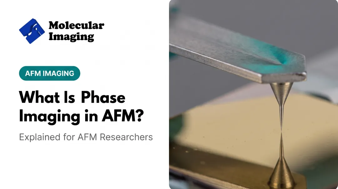
- Choose tip geometry by what you're measuring. Sharp tips resolve fine adhesion sites; colloidal probes give cleaner Hertzian fits on soft, uneven samples like cells.
- Molecular Imaging's contact-mode and liquid-environment cantilevers cover both ends of this range, with diamond-coated probes available for indentation on harder materials.
Step 2 – Calibrate the System
- Determine deflection (light lever) sensitivity first, using a curve on an incompressible surface such as mica or a gold-on-mica substrate.
- Calibrate the actual spring constant with the thermal noise method or the Sader method rather than trusting the number printed on the box.
- NIST has documented cases where a cantilever's real stiffness differs from its stated value by a factor of two, enough to throw off every modulus calculated afterward.
- Molecular Imaging supplies mica, gold-on-mica, and periodic grating calibration standards built for exactly this step.
Step 3 – Measure the Curve or Force Map
Run the approach-retract cycle in contact mode. For statistically meaningful results, collect a grid of curves across the sample—force volume or force mapping—rather than relying on a single point.
Review a handful of single curves before you commit to a full map. Force maps take hours to re-run, so catching a bad setup early saves the whole session.
Step 4 – Process Raw Data
- Convert deflection voltage to force using the sensitivity factor from Step 2.
- Correct any tilted baseline before extracting values, ideally in force-time space so the fix stays consistent across the entire curve.
- Identify the exact contact point, the transition where the probe stops responding only to long-range forces and starts indenting the sample.
Step 5 – Apply a Contact Mechanics Model
Fit the loading curve with a model that matches your tip geometry and indentation depth:
| Model | Best fit for |
|---|---|
| Hertz | Spherical or colloidal tip, shallow indentation |
| Sneddon | Conical or pyramidal tip, deeper indentation |
| DMT | Adhesive contact on stiffer materials |
| JKR | Adhesive contact on softer materials |
Model choice isn't a rounding error. Published comparisons have shown a blunted pyramidal tip modeled as an ideal cone can overestimate modulus by 100%.
Calculate adhesion force and work of adhesion separately, from the area under the retract curve's pull-off dip.
Step 6 – Interpret, Validate, and Iterate
- Compare extracted values against literature or expected ranges for the material.
- Discard curves distorted by drift, contamination, or an ambiguous contact point. Don't average them into good data.
- Refine parameters on a small batch before scaling up to automated mapping across dozens or hundreds of points.

Common Force Curve Artifacts & Troubleshooting
Non-ideal curves are the norm, not the exception. Spotting them early keeps flawed conclusions out of papers and grant reports.
As noted earlier, one 2025 study pooling multiple AFM datasets rejected nearly 30% of curves—for reasons from pre-contact drift to ambiguous contact points. That rate is from one heterogeneous dataset, not a universal benchmark, but it shows how often artifacts appear even in careful work.
| Artifact | Likely cause | What to do |
|---|---|---|
| Tilted baseline | Laser interference, poor grounding, thermal drift | Apply a baseline-fitting correction to the flat, non-contact region |
| Discontinuity on approach | Often a real event, such as puncturing a lipid bilayer | Confirm against expected sample structure before assuming error |
| Multiple pull-off events | Sequential bond breakage in cell-cell or receptor-ligand studies | Analyze each rupture separately instead of averaging |
| Transient spikes or noise | Debris or floating particles crossing the laser path in liquid | Discard the curve and rerun under cleaner conditions |
Best practice: Always collect and review a few single-point curves before launching a full automated force map. Maps can take hours; catching a bad parameter early saves the entire run.
How Molecular Imaging Can Help
Force spectroscopy is only as good as the instrument running it. Molecular Imaging builds its AFM and BioAFM platforms around modular scanner heads that switch between imaging and force measurement without swapping systems — including the 5500 ILM PicoPlus BioAFM, 5500 PicoPlus AFM+STM, and 5420 PicoAFM.
A few features matter specifically for force curve work:
- Calibration standards — mica, gold-on-mica, and periodic gratings give flat, well-characterized surfaces for deflection sensitivity and spring constant checks
- MAC Mode on the 5500 ILM PicoPlus BioAFM — magnetic AC drive cuts fluid-coupling noise that plagues conventional tapping in liquid, useful for cell-cell and receptor-ligand adhesion studies
- Environmental control — temperature-controlled stages (-30°C to 250°C) and isolation chambers hold humidity, temperature, and gas composition steady during long mapping sessions
- Application support — former instrument engineers staff the team, with a video tutorial library that includes a dedicated Force Curve session on acquisition and troubleshooting

For labs running an aging or malfunctioning system, ZoomAFM Fast Online Service provides remote diagnostics, calibration support, and repair, so a sticky pull-off measurement doesn't turn into weeks of downtime.
Conclusion
Force-distance curves give researchers something topography alone cannot: a direct read on how a sample behaves under load, down to a single molecule or a single membrane. That value depends entirely on getting the fundamentals right: matched probes, verified calibration, and a clear eye for artifacts before they get baked into a dataset.
Treat calibration as a habit, not a one-time setup. A cantilever that behaved predictably on your last sample may respond differently on a new substrate or a different buffer. Revisit the basics with each new project, and force curves become a reliable, high-precision measurement—not a source of doubt.
Frequently Asked Questions
How does AFM measure force?
AFM measures force through cantilever deflection, detected by a laser reflecting onto a photodetector. That signal is converted into force units using the calibrated spring constant and deflection sensitivity.
What is a force curve?
A force curve is a plot of tip-sample interaction force against probe-sample separation, recorded as the cantilever approaches and then retracts from a surface at a single point.
What are the forces involved in AFM?
Long-range forces, including van der Waals, electrostatic, and capillary, act before contact. Contact brings repulsive loading forces, while retraction reveals the adhesive forces holding the tip to the surface.
What is the difference between a force curve and force spectroscopy?
A force curve is one approach-retract measurement at a single point. Force spectroscopy is the broader technique of collecting and analyzing many such curves to study interactions statistically.
How do you interpret an AFM force-distance curve?
Locate the contact point, then fit the loading segment to a mechanical model for stiffness. On the retract curve, measure the adhesion dip for binding force and energy.
What causes errors in AFM force-distance curves?
Common causes include incorrect calibration, thermal drift, tilted baselines, and contamination in the fluid or air path. Careful setup and environmental control resolve most of them.