
Many researchers get stuck comparing AM-AFM and FM-AFM without a clear framework for which one fits their sample. Pick the wrong mode, and you either damage a delicate biological specimen or fail to reach the resolution your experiment demands.
This article breaks down what Frequency Modulation AFM actually is, how its feedback loop works, and when it makes sense over Amplitude Modulation AFM.
Key Takeaways
- FM-AFM tracks cantilever resonance frequency shifts, not amplitude, for high-sensitivity force detection
- Excels at atomic-resolution imaging in ultra-high vacuum and gentle imaging of soft samples
- Requires phase-locked loop (PLL) electronics, adding complexity versus AM-AFM
- Match the mode to sample rigidity, environment, and resolution needs
What Is Frequency Modulation Atomic Force Microscopy?
FM-AFM is a dynamic AFM mode where the cantilever oscillates at its resonance frequency, and shifts in that frequency become the imaging signal.
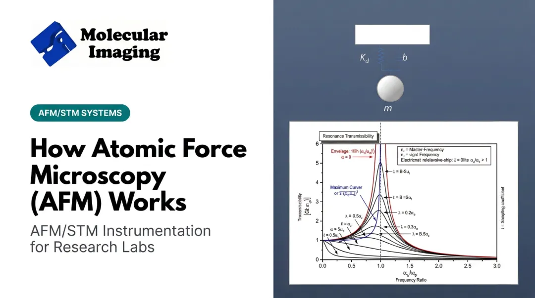
Here's the core principle: as the tip approaches a sample, attractive or repulsive forces change the effective stiffness of the cantilever. That stiffness change shifts the resonant frequency. A phase-locked loop (PLL) demodulator tracks this shift in real time and feeds it back as the control signal.
Albrecht and colleagues introduced frequency-modulation force detection in 1991, designing it to exploit high-Q cantilevers for better sensitivity without sacrificing bandwidth (Albrecht et al., 1991). A few years later, Giessibl used noncontact FM-AFM to image the reconstructed Si(111)-(7×7) surface at atomic resolution (Giessibl, 1995, Science).
This is fundamentally different from AM-AFM, better known as tapping mode. AM-AFM watches the oscillation amplitude drop as the tip nears the surface. FM-AFM watches the frequency shift instead — a distinction that shapes imaging speed, force sensitivity, and which environments the mode handles well.
How Frequency Modulation AFM Works: The Technical Mechanism
FM-AFM runs on a closed feedback loop with several coordinated pieces:
- Self-excitation circuit — keeps oscillation amplitude constant using an automatic gain controller, isolating frequency shift as the sole force-sensitive variable.
- Phase-locked loop (PLL) tracking — continuously demodulates the tip-sample interaction, generating a real-time frequency-shift signal.
- Z-feedback controller — compares the measured frequency shift against a setpoint and adjusts tip-sample distance to hold it constant.

This separation matters. In AM-AFM, both amplitude and phase changes feed into the response, but that response is inherently slower and tied to how quickly amplitude can settle.
FM-AFM's frequency tracking responds nearly instantaneously. That speed is especially valuable for high-Q cantilevers under vacuum, where amplitude changes decay slowly.
Why Q Factor Matters
In ultra-high vacuum, cantilevers can reach extremely high Q values, meaning very low energy dissipation and very sharp resonance peaks. The original FM design specifically exploited this: higher Q gives better force-gradient sensitivity without the bandwidth penalty that plagues simple amplitude-slope detection.
That sensitivity supports true non-contact operation. FM-AFM keeps the tip far enough from the surface to avoid damaging reactive or fragile samples while still resolving atomic-scale force gradients.
If you're setting up an FM-AFM system, expect to work with:
- An oscillator/self-excitation module
- A PLL demodulator
- An amplitude controller
- A Z-feedback loop
Ask your instrument vendor for the specific electronic block diagram for your setup — architectures vary between manufacturers.
Frequency Modulation vs. Amplitude Modulation AFM
What is the difference between AM and FM modulation modes in practice?
In practice, the two modes differ across signal type, operating environment, Q-factor needs, system complexity, and typical use:
| Factor | FM-AFM | AM-AFM |
|---|---|---|
| Signal tracked | Frequency shift (force gradient) | Oscillation amplitude |
| Best environment | Ultra-high vacuum | Air, liquid |
| Q-factor need | Thrives on very high Q | Works fine at lower Q |
| Complexity | Higher (PLL required) | Lower |
| Typical use | Atomic resolution, non-contact | Routine topography, biological samples |

FM-AFM's near-instant frequency detection makes it ideal where cantilever Q is extremely high, which is exactly what vacuum conditions provide. AM-AFM's slower amplitude response is actually an advantage in air and liquid, where damping keeps Q naturally lower and amplitude settling is fast enough to be practical.
Is AM-AFM still used today?
Yes, overwhelmingly so. AM-AFM (tapping mode) remains the most common AFM mode in everyday labs. Bruker calls it their most popular mode because it is simpler and more robust in air and liquid. It also skips the extra electronics FM-AFM requires (Bruker TappingMode).
FM-AFM stays reserved for specialized cases: atomic-resolution surface science, quantitative force-gradient measurements, and non-contact imaging of reactive or fragile materials.
Key Applications of Frequency Modulation AFM
FM-AFM is used where high force sensitivity and true non-contact operation matter most.
For atomic and molecular-resolution surface imaging, its UHV pedigree suits crystal surfaces, semiconductors, and thin films where individual atoms must be resolved. Giessibl's Si(111) work remains a benchmark; later studies extended atomic-resolution FM imaging to metal surfaces such as Ag(111).
In molecular electronics, researchers studying charge transport at nanoscale junctions combine FM-AFM with simultaneous electrical measurement. One study imaged DNA on copper substrates while tracking electron transfer; later work used frequency-shift steps to identify molecular charge-state changes.
Force spectroscopy is another strength. FM-AFM probes individual chemical bonds for strength and angular dependence at the site-specific level. Amplitude-based methods cannot reach this regime.
Materials science applications include:
- Battery interface research (for example, an electrolyte reaction field near a negative electrode in a lead-acid setup)
- Polymer in-plane mechanics using frequency-modulated torsional resonance techniques
- Reactive surface studies that track on-surface chemical reactions atom by atom

Molecular Imaging's 5500 PicoPlus platform family supports work across several of these areas, including polymer analysis, semiconductor research, and lithium-ion battery studies. Modular configurations and environmental control cover humidity, temperature, and gas atmosphere.

Advantages, Limitations, and Choosing the Right AFM System
FM-AFM brings clear gains in some labs and real trade-offs in others. Matching the mode to your sample and environment matters more than defaulting to one technique.
FM-AFM advantages:
- Higher force sensitivity through direct force-gradient measurement
- True non-contact operation, minimizing tip-induced damage
- Superior resolution on stiff, rigid samples in vacuum
FM-AFM limitations:
- Requires PLL and self-excitation electronics, adding cost and setup complexity
- Less practical for soft biological samples in liquid, where low Q-factor increases frequency noise
- AM/tapping modes generally outperform it for routine, high-throughput topography
Choosing between FM and AM comes down to three questions:
- What's your sample? Rigid crystal or reactive surface → choose FM. Soft biomolecule or polymer film → choose AM.
- What's your environment? Vacuum → FM is strongest. Air or liquid → AM is usually the practical choice.
- What resolution do you actually need? Atomic-scale force gradients demand FM. Routine topography rarely does.
Once those answers are clear, pick a platform that can run the mode your work actually needs.
Molecular Imaging's modular AFM/STM systems, including the 5500 PicoPlus AFM+STM and 5500 ILM PicoPlus BioAFM, support multi-frequency operation and flexible imaging-mode setups. Researchers in nanotechnology, life sciences, and materials science can reconfigure as experiments change.
Technical documentation and direct support are available at 1-888-644-0389.
Frequently Asked Questions
What is frequency modulation in AFM and how is it used?
FM-AFM measures shifts in cantilever resonance frequency caused by tip-sample force gradients. It's used mainly for non-contact, atomic-resolution imaging in ultra-high vacuum environments.
Is AM-AFM still used today?
Yes. AM-AFM (tapping mode) remains the dominant mode for everyday imaging in air and liquid, thanks to its simplicity and robustness compared to FM-AFM's more complex electronics.
What is the difference between AFM and MFM?
AFM measures general surface topography through mechanical tip-sample forces. Magnetic Force Microscopy (MFM) is a specialized AFM mode that maps magnetic field gradients above a sample's surface.
Can FM-AFM be used in liquid environments?
Technically, yes, but it's less common. Liquid loading lowers the cantilever's Q-factor, increasing frequency noise, which makes AM-AFM the more practical choice for most liquid and biological imaging.
What equipment is required to perform FM-AFM?
You need a PLL demodulator, a self-excitation oscillator circuit to maintain constant amplitude, and a cantilever suited for tracking high-Q resonance shifts reliably.
How does FM-AFM achieve atomic resolution?
In ultra-high vacuum, the cantilever's very high Q-factor allows extremely sensitive detection of tiny frequency shifts, each corresponding to individual atomic-scale force interactions between tip and sample.