
Force Volume Mapping (FVM) solves this by turning an AFM tip into a nanoscale mechanical probe at every pixel. Instead of one image, you get a full grid of force-distance curves, each one a window into local stiffness, adhesion, and deformation.
This article covers how FVM works, where it's used across materials science, biology, and battery research, and what to look for in an AFM system built for serious force spectroscopy work.
Key Takeaways
- FVM captures a full force-distance curve at each grid point, mapping stiffness, adhesion, and deformation with topography
- Use cases include polymer blends, live-cell mechanics, and battery SEI characterization
- Grid resolution and acquisition time trade off directly: a 1,024-point map can take 20–30 minutes
- Match the contact model (Hertz, DMT, Sneddon) to probe geometry—or modulus values are meaningless
- Liquid-cell and environmental control on modular AFM platforms improve force-volume reproducibility
What Is Force Volume Mapping?
Force volume mapping (FVM) is a technique where the AFM tip performs a full approach-retract force curve at every pixel across a defined grid. The result is a three-dimensional dataset: force versus tip-sample separation, repeated across x-y space.
That's the core distinction from standard AFM imaging. Regular tapping-mode imaging gives you height. FVM gives you height plus a quantitative mechanical fingerprint at every location.
From each curve, you can extract:
- Elastic modulus/stiffness — how much the sample resists deformation
- Adhesion — the pull-off force as the tip retracts
- Deformation — how far the tip indents the sample under load
- Dissipation — energy lost during the contact cycle
FVM vs. PeakForce QNM
PeakForce QNM is a related, faster technique. It analyzes one force curve per tap while scanning at speeds close to standard tapping mode, producing the same property channels. Classical FVM, by contrast, captures a slower, more complete curve at each point. According to Bruker, conventional force-volume acquisition often takes about one second per curve and several hours for a full useful image. PeakForce QNM trades some per-curve detail for speed.
FVM traces back to early 1990s AFM development. Automated force-volume imaging methods were documented for applications ranging from protein adhesion mapping to living-cell microelasticity studies, establishing the technique long before faster derivatives arrived.
How Force Volume Mapping Works
At each XY grid point, the cantilever approaches, contacts, and retracts from the surface while deflection is continuously recorded. That raw deflection-versus-piezo-position data gets converted into force versus separation.
Fitting the Contact Mechanics Model
The contact portion of the curve is fit against a model matched to probe geometry:
| Model | Best for | Key limitation |
|---|---|---|
| Hertz | Spherical probes, no adhesion assumed | Doesn't account for adhesive pull-in |
| DMT | Spherical/parabolic tips with adhesion | Excludes viscoelastic effects |
| Sneddon | Conical or pyramidal tips | Purely elastic assumption |

Getting this wrong produces numbers that look precise but mean nothing. Modulus values calculated with mismatched models aren't comparable to each other.
Calibration Matters More Than People Think
Cantilever spring constant, tip radius, and deflection sensitivity all feed directly into the force calculation. Bruker's own uncertainty analysis attributes roughly 15% error from tip radius alone, 6-16% from spring constant, and about 5% from deflection sensitivity. Uncalibrated systems can produce modulus values off by a third or more.
Resolution vs. Time
Higher pixel density means finer spatial detail, but every additional point adds acquisition time. A well-documented example: a 32×32 grid (1,024 curves) over a 5×5 µm area took roughly 20-30 minutes in a peer-reviewed study. Push resolution higher, and hours can pass before a single map completes.

Once the grid is collected, software stitches those curves into 2D channels for stiffness, adhesion, and deformation. Molecular Imaging's PicoView is built for that load, with volume spectroscopy, FlexGrid spectroscopy, and advanced force mapping workflows.
Environmental Stability Isn't Optional
Temperature drift and humidity changes shift cantilever baseline readings mid-scan, corrupting long acquisitions. Molecular Imaging's temperature-controlled stages (rated -30°C to 250°C) and Environmental Isolation Chambers address this directly. They hold humidity, temperature, and gas atmosphere steady across extended force volume sessions, which matters for battery and polymer studies that run for hours.
Applications of Force Volume Mapping
Materials Science
FVM excels at revealing mechanical heterogeneity that would otherwise stay hidden. A 2021 study on polyolefin elastomer blends mapped polystyrene mixed with low-density polyethylene using both PeakForce QNM and fast force volume, tracking DMT modulus and dissipation channels.
The reported modulus varied from 11.7 MPa at low frequency to 89.6 MPa at 2 kHz — a reminder that acquisition frequency itself changes what you measure.

Life Sciences
BioAFM applications extend force mapping to live cells and biomolecules in liquid. Studies on CHO cells found that raised surface features like microvilli correlated with measurably higher local stiffness.
Red blood cell mapping identified spectrin fiber structures through mechanical contrast alone.
Battery and Electrochemistry Research
SEI (solid electrolyte interphase) layers on lithium metal are notoriously hard to characterize with topography alone. In-situ AFM studies using PeakForce QNM tracked SEI stiffness evolution over hours, finding stiffness shifts from near 0 GPa up to 11.2 GPa as the SEI matured.
Electrolyte additives like VC produced more heterogeneous, evolving mechanical profiles. That temporal mechanical mapping simply is not available from height images alone.

Best Practices for Accurate Force Volume Mapping
Reproducible force volume maps come down to three fundamentals:
- Match cantilever stiffness to sample hardness. A cantilever too stiff for a soft polymer or cell membrane won't register meaningful deflection. One too soft against a hard sample risks tip damage.
- Calibrate before every session. Deflection sensitivity and spring constant drift over time and between mounts — don't reuse yesterday's calibration.
- Balance grid density against acquisition time. A denser grid gives more spatial detail but can turn a 20-minute scan into a multi-hour one.
Molecular Imaging's cantilever lineup spans the stiffness range these measurements need:
- Soft samples: FM-10 (low-frequency soft tapping) or MAC Levers Types V-VII for DNA and proteins in liquid
- General use: NCL-30-10 or MAC Lever Type I for air/liquid versatility
- Stiffer samples: MAC Lever Type II or NCH-30-10
- Direct mechanical testing: ContSi-10 or the diamond-coated Diamond-10 for indentation and wear studies
Choosing the Right AFM System for Force Volume Mapping
Force volume work demands a platform that doesn't lock you into one measurement mode. Look for:
- Interchangeable probe/nose-cone configurations that switch between AFM, STM, and force-measurement modes without a full system rebuild
- Liquid-cell compatibility for biological or electrochemical samples
- Environmental accessories for temperature- and atmosphere-controlled experiments
Molecular Imaging's 5420 PicoAFM offers interchangeable nose cones for switching between imaging and force techniques. The 5500 PicoPlus AFM+STM and 5500 ILM PicoPlus BioAFM extend this further. The BioAFM variant is purpose-built for liquid-environment force mapping on cells and biomolecules, with sub-angstrom lateral resolution and scan ranges up to 90 µm × 90 µm.

For labs running older Agilent-era systems, ZoomAFM provides diagnostics, calibration, and repair support so existing force volume workflows don't grind to a halt over a failing controller or misaligned photodetector.
Frequently Asked Questions
What is the difference between force volume mapping and force spectroscopy?
Force spectroscopy is a single point measurement: one or a few force curves at chosen locations. Force volume mapping repeats that measurement across a full grid, generating a spatial map of mechanical properties rather than a single data point.
How long does a typical force volume scan take?
It depends heavily on grid resolution. A 32×32 grid (1,024 points) typically takes about 20–30 minutes; denser grids or slower curve settings can stretch into hours.
Can force volume mapping be used on biological samples in liquid?
Yes. BioAFM-compatible systems, like Molecular Imaging's 5500 ILM PicoPlus, support force mapping on live cells and biomolecules under physiological liquid conditions.
What software is used to analyze force volume data?
AFM manufacturers typically provide proprietary software with built-in contact mechanics fitting. Molecular Imaging's PicoView software supports volume spectroscopy, FlexGrid spectroscopy, and advanced force mapping workflows.
How does cantilever choice affect force volume mapping results?
Spring constant and tip geometry directly determine measurement sensitivity. A mismatched cantilever (too stiff or too soft for the sample) produces inaccurate stiffness and adhesion readings, or risks damaging the tip.
Is force volume mapping the same as PeakForce Tapping?
No. PeakForce Tapping is a faster, related technique that also generates a force curve per pixel, but at much higher scan speeds. It trades some per-curve detail for much shorter acquisition times.