
Scanning Microwave Impedance Microscopy (sMIM) fills that gap. It's an AFM-based technique that pairs GHz-frequency microwave reflectometry with a shielded probe, producing simultaneous maps of topography, conductance, and capacitance, all non-destructively.
This article walks through where sMIM is actually being used today: semiconductor failure analysis, dopant profiling, twisted 2D materials and quantum systems, and the emerging frontier of biological imaging.
Key Takeaways
- Maps conductivity (MIM-Re) and capacitance (MIM-Im) with AFM topography in one non-destructive pass
- Enables dopant profiling, buried defect detection, 2D domain imaging, and quantum capacitance studies
- Resolution spans ~100 nm with standard tips to sub-nanometer with liquid immersion
- Control humidity, stray capacitance, and tip condition to keep results reliable
- Modular AFM platforms with environmental control make electrical-imaging workflows more reproducible
What Is Scanning Microwave Impedance Microscopy?
Scanning microwave impedance microscopy (sMIM) is an AFM-based technique that maps local electrical impedance at the nanoscale. It sends a microwave signal, typically around 2.9–3.0 GHz, through a shielded AFM probe and reads the reflected signal at the tip-sample junction (Zheng et al., 2020).
That junction behaves like a small impedance circuit. As the probe scans, the reflected wave is demodulated into two channels:
- MIM-Re (real/resistive component) — tracks local conductance
- MIM-Im (imaginary/capacitive component) — tracks local capacitance and dielectric variation
For quantitative work, researchers model the tip as a compact RLC network—about 1 Ω resistance, 0.16 pF capacitance, and 10 nH inductance near 1 GHz—then use a matching network to convert simulated admittance into calibrated MIM-Re and MIM-Im values.

Why Resolution Isn't Limited by Wavelength
A 3 GHz signal has a free-space wavelength of roughly 0.1 meters, yet sMIM regularly resolves features thousands of times smaller. Spatial resolution comes from near-field confinement at the tip apex, not the free-space wavelength.
Conventional tips confine the field to roughly 50–100 nm. Conditioned tips and liquid-meniscus techniques push that confinement much further, so published resolution figures depend heavily on probe preparation and operating setup.
Applications in Semiconductor & Dopant Characterization
Semiconductor labs were early adopters of sMIM because it solves a genuine problem: seeing dopant distribution and buried structures without cutting the wafer apart.
NIST researchers combined an AFM probe with a vector network analyzer operating across 1–20 GHz and successfully profiled silicon dopant concentrations spanning 10¹⁴ to 10²⁰ atoms/cm³, with roughly 20% relative error (NIST, 2012). That same study imaged p-n junction interfaces and nanoscale defect structures, pointing directly to failure-analysis use.
Buried structure detection has real limits, though. A benchmark study using 10 nm-wide phosphorus-doped silicon lines buried about 30 nm below the surface found the minimum resolvable line separation was 76–88 nm; anything tighter than roughly 64 nm went undetected.

Practical applications include:
- Dopant/carrier profiling across wafer cross-sections without destructive prep
- Buried defect and junction mapping for IC failure analysis
- Dielectric thin-film characterization — oxide thickness, permittivity, and quantitative constants via finite-element analysis
- Process control feedback — quantitative capacitance imaging gives fabrication teams a non-destructive check on film uniformity
Building a reliable conductive/capacitive imaging workflow requires the right hardware foundation. Molecular Imaging's modular AFM/STM platforms, including the 5500 PicoPlus series, let researchers combine conductive AFM with interchangeable scanner configurations.
Modular conductive AFM options let labs customize advanced electrical imaging setups instead of locking into a single fixed-purpose tool.
Applications in 2D Materials, Moiré Superlattices & Quantum Research
Twisted 2D materials are where sMIM has produced some of its most striking images. Twist angle and layer stacking create moiré superlattices with electronic properties that shift dramatically over just a few nanometers, exactly the scale sMIM is built for.
A 2020 study imaged twisted double-bilayer graphene and measured a moiré period of 10.9 ± 0.7 nm at a twist angle of 1.3 ± 0.1 degrees, achieving sub-5-nm resolution after tip conditioning (Zheng et al., Science Advances, 2020).
Pushing Resolution with Liquid Immersion
A separate technique uses a water meniscus to concentrate the microwave near-field around the tip. This immersion approach reported resolution better than 1.05 nm while still operating near 3 GHz — a wavelength-to-resolution ratio described as 10⁸ (Wu et al., Nature Communications, 2021).

The same paper notes that single-layer talc or hBN sheets can serve as coverslips thin enough for microwave transmission, a detail that later supports biological work.
Quantum Capacitance and Nanotube Mapping
sMIM also maps quantum capacitance, where microwave reflectivity tracks local density of states rather than geometry alone. A 2016 ACS Nano study on single-wall carbon nanotubes reported:
- Reflectivity tied directly to quantum capacitance
- Local impedance and density-of-states maps in one pass
- Lateral resolution below 50 nm
The same contrast modes help in battery and energy-storage electrode work. Local conductivity swings at grain boundaries shape performance, yet standard AFM often misses them.
Applications in Life Sciences & Biological Imaging
Biological sMIM is still a research frontier. The core challenge: biological samples live in liquid, and liquid environments introduce dielectric loss and meniscus instability that complicate microwave measurements.
One proposed solution is imaging through microwave-transparent window materials. A 2016 NIST study described imaging liquids through ultra-thin dielectric membranes only a few nanometers thick (Tselev et al., 2016).
Those membranes are transparent enough to microwaves to support in-situ study of biological or reactive samples while isolating the probe from the liquid. Single-layer hBN or talc has been proposed as a coverslip material for this purpose.
Potential applications include:
- Probing membrane conductivity in near-native liquid conditions
- Mapping biomolecular electrical properties without fixing or drying samples
- Studying ionic transport across membranes at nanoscale resolution
Current limitations remain significant:
- Water's high relative permittivity at GHz frequencies must be carefully modeled
- Meniscus behavior shifts with humidity and temperature
- No published study yet provides a universal biological-window resolution benchmark
A 2025 review confirms sMIM can characterize tissues and single cells but stops short of quantifying routine performance (APL Materials, 2025).
For labs approaching this from the AFM side rather than pure sMIM, Molecular Imaging's 5500 ILM PicoPlus BioAFM already supports in-liquid imaging through MAC Mode and a range of liquid-cell designs. That same foundational hardware is what bio-electrical imaging research tends to build on.
Advantages, Limitations & Choosing the Right AFM System
Where sMIM Wins
- Non-destructive — no cross-sectioning, no sample damage
- Quantitative — admittance-based signals can be calibrated against known dielectric standards
- Ambient operation — works in air at room temperature, no vacuum chamber required, unlike electron-based techniques
Where It Struggles
- Humidity sensitivity — water meniscus formation depends on humidity, temperature, and tip velocity, altering effective resolution regardless of tip geometry
- Stray capacitance — parasitic capacitance from cabling and probe geometry requires careful artifact subtraction
- Force control — consistent tip-sample contact is essential for repeatable admittance readings
A 2025 review of the technique explicitly flags rough-surface effects and complex field distributions as ongoing sources of measurement uncertainty. None of this means sMIM is unreliable, but it does mean the surrounding instrument matters as much as the probe itself.
Reliable electrical imaging depends on stable environmental conditions and modular hardware that can be reconfigured as experiments evolve. Molecular Imaging offers:
- Environmental Isolation Chambers for the 5500 PicoPlus, controlling humidity, temperature, and gas conditions
- Temperature-controlled sample stages spanning −30°C to 250°C, useful for stabilizing surface moisture behavior
- Modular scanner architecture supporting AFM, STM, CSAFM, KPFM, EFM, and MFM configurations without swapping the entire microscope
For labs building custom conductivity or capacitance imaging workflows, that modularity, backed by ZoomAFM technical support, matters more than any single spec sheet.
Frequently Asked Questions
What is the difference between MIM-Re and MIM-Im signals?
MIM-Re captures the real, resistive component of the reflected microwave signal, corresponding to local conductance. MIM-Im captures the imaginary component, which reflects capacitance and dielectric variation.
What resolution can scanning microwave impedance microscopy achieve?
Conventional tip geometries typically resolve down to 50–100 nm. Conditioned tips have reached sub-5-nm resolution, and liquid-immersion techniques have demonstrated better than 1.05 nm in published studies.
How is sMIM used in semiconductor failure analysis?
It maps dopant concentration and carrier profiles without destructive cross-sectioning, and it has been used to identify buried defects, p-n junctions, and leakage pathways in integrated circuits.
Can sMIM be used on biological samples?
This remains an active research area. Researchers are exploring microwave-transparent membranes, including hBN and talc, to image biological samples in liquid without direct probe contact.
What are the main limitations of microwave impedance microscopy?
Humidity and meniscus instability can shift effective resolution, and stray capacitance from cabling and probe geometry requires careful compensation during measurement setup.
How does sMIM compare to other nanoscale imaging techniques like TERS or s-SNOM?
s-SNOM and TERS use optical scattering or Raman signals at visible wavelengths, typically at 10–100 nm resolution. sMIM measures microwave-frequency admittance, so it reports conductivity and capacitance directly rather than optical contrast.